Optimizing Embeddings
Learn how to optimize embedding models for better retrieval in RAG systems—covering model selection, dimensionality, and domain-specific tuning.
In this cookbook, we demonstrate how to fine-tune open-source embedding models using sentence-transformer and then evaluating its performance. Like always, we’ll focus on data-driven approaches to measure and improve retrieval performance.
Imagine you’re building a dating app. Two users fill in their bios:
- “I love coffee.”
- “I hate coffee.”
From a linguistic standpoint, these statements are opposites. But from a recommendation perspective, there’s a case to be made that they belong together. Both are expressing strong food preferences. Both might be ‘foodies’ which is why they mentioned their preferences.
The point here is subtle, but important: semantic similarity is not the same as task relevance. That’s why fine-tuning your embedding model, even on a small number of labeled pairs, can make a noticeable difference. I’ve often seen teams improve their recall by 10-15% by fine-tuning their embedding models with just a couple hundred examples.
Requirements
Before starting, ensure you have the following packages installed:
Setup
Start by setting up LangWatch to monitor your RAG application:
Generating Synthetic Data
In this section, we’ll generate synthetic data to simulate a real-world scenario. We’ll mimic Ramp’s successful approach to fine-tuning embeddings for transaction categorization. Following their case study, we’ll create a dataset of transactions objects with associated categories. I’ve pre-defined some categories and stored them in data/categories.json. Let’s load them first and see what they look like.
Let’s now create a Pydantic Model to represent the transaction data. Following their casestudy, each transaction will be represented as an object containing:
- Merchant name
- Merchant category (MCC)
- Department name
- Location
- Amount
- Memo
- Spend program name
- Trip name (if applicable)
Notice that I don’t include the expense_category in the format_transaction method, since this is our label. Now that we have a Transaction class, let’s load the data and create our evalset. I’ll use the instructor library to generate data in the format we need.
We can now generate a large number of transactions using asyncio and our generate_transaction function.
Awesome. Now let’s create a list of transactions, where each transaction is a dictionary with a “query” and “expected” key.
Setting up a Vector Database
Let’s set up a vector database to store our embeddings of categories.
Parametrizing our Retrieval Pipeline
The key to running quick experiments is to parametrize the retrieval pipeline. This makes it easy to swap different retrieval methods as your RAG system evolves. Let’s start by defining the metrics we want to track.
Recall measures how many of the total relevant items we managed to find. If there are 20 relevant documents in your dataset but you only retrieve 10 of them, that’s 50% recall.
Mean Reciprocal Rank (MRR) measures how high the first relevant document appears in your results. If the first relevant document is at position 3, the MRR is 1/3.
The case for recall is obvious, since it’s the main thing you’d want to track when evaluating your retrieval performance. The case for MRR is more subtle. In Ramp’s application, the end-user is shown a number of categories for their transaction and is asked to pick the most relevant one. We want the first category to be the most relevant, so we care about MRR.
Sidenote: You don’t need 100 different metrics. Think about what you care about in your application and track that. You want to keep the signal-to-noise ratio high.
Before we move on to define both the retrieval function and the evaluation function, let’s first structure our data.
Let’s first create a training and evaluation set, so that we can evaluate the performance when we fine-tune our embedding model later fairly.
Now we can set up our parametrized retrieval pipeline. I’ll vary the number of retrieved documents to see how it affects recall and MRR. Note that you can easily vary other parameters (like the embedding models or rerankers) as well with this parametrized pipeline.
Fine-tune embedding models
Moving on, we’ll fine-tune a small open-source embedding model using just 256 synthetic examples. It’s a small set for the sake of speed, but in real projects, you’ll want much bigger private datasets. The more data you have, the better your model will understand the details that general models usually miss.
One big reason to fine-tune open-source models is cost. After training, you can run them on your own hardware without worrying about per-query charges. If you’re handling a lot of traffic, this saves a lot of money fast.
We’ll be using sentence-transformers — it’s easy to train, plays nicely with Hugging Face, and has plenty of community examples if you get stuck. Let’s first transform our data in the format that sentence-transformer expects it.
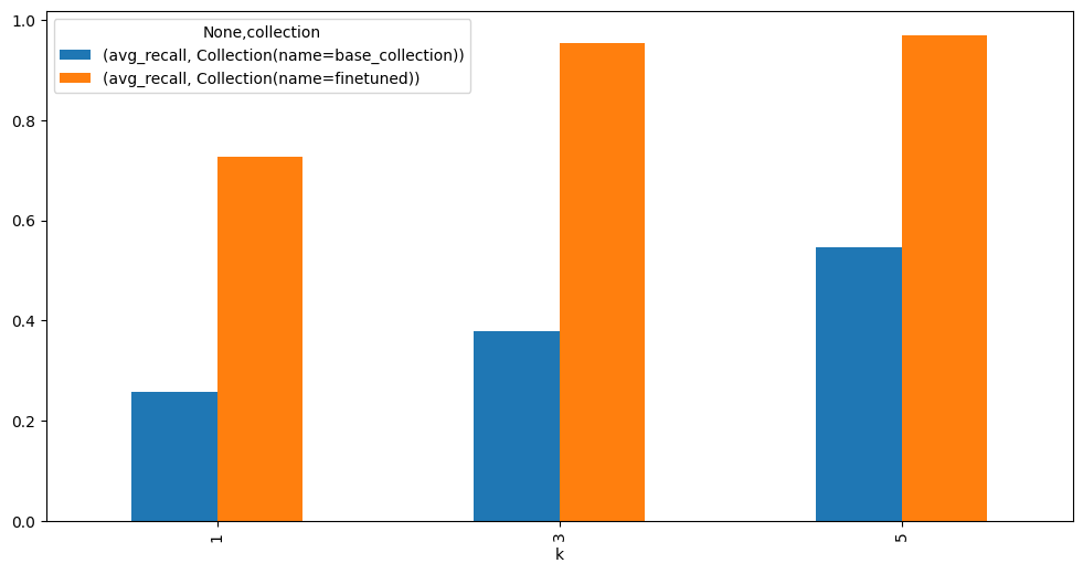
We’ll use the MultipleNegativesRankingLoss to train our model. This loss function works by maximizing the similarity between a query and its correct document while minimizing the similarity between the query and all other documents in the batch. It’s efficient because every other example in the batch automatically serves as a negative sample, making it ideal for small datasets.
Now we can start training. If you’re done training, you can optionally upload it to HuggingFace.
Now we can create a new collection using our fine-tuned embedding model.
Let’s compare the performance of the two models using our parametrized retrieval pipeline.
Conclusion
We see that the fine-tuned model performs better than the base model on the evaluation set. Like I said at the beginning of this post, I often find teams improve their retrieval significantly by fine-tuning embedding models on their specific data, for their specific application. Note that we didn’t even need that much data. A few hundred examples is often enough.
For the full notebook, check it out on: GitHub.